Beer Markets – Ryan Horn’s Website

Here is some analytics in relation to Beer Markets!

── Attaching core tidyverse packages ──────────────────────── tidyverse 2.0.0 ──
✔ dplyr     1.1.4     ✔ readr     2.1.4
✔ forcats   1.0.0     ✔ stringr   1.5.0
✔ ggplot2   3.4.4     ✔ tibble    3.2.1
✔ lubridate 1.9.3     ✔ tidyr     1.3.0
✔ purrr     1.0.2     
── Conflicts ────────────────────────────────────────── tidyverse_conflicts() ──
✖ dplyr::filter() masks stats::filter()
✖ dplyr::lag()    masks stats::lag()
ℹ Use the conflicted package (<http://conflicted.r-lib.org/>) to force all conflicts to become errors
Rows: 73115 Columns: 26
── Column specification ────────────────────────────────────────────────────────
Delimiter: ","
chr (15): X_purchase_desc, brand, container, region, state, market, buyertyp...
dbl  (5): household, quantity, dollar_spent, beer_floz, price_floz
lgl  (6): promo, childrenUnder6, children6to17, microwave, dishwasher, singl...

ℹ Use `spec()` to retrieve the full column specification for this data.
ℹ Specify the column types or set `show_col_types = FALSE` to quiet this message.

# A tibble: 1 × 3
  avg_price avg_spent avg_volume
      <dbl>     <dbl>      <dbl>
1    0.0560      13.8       266.

These values summarize average price per ounce, spending, and purchase volume across all households.

# A tibble: 5 × 2
  brand             n
  <chr>         <int>
1 BUD_LIGHT     21592
2 MILLER_LITE   17159
3 COORS_LIGHT   13074
4 NATURAL_LIGHT 12616
5 BUSCH_LIGHT    8674

This shows which brands are purchased most frequently.

# A tibble: 2 × 3
  promo avg_price pct_diff
  <lgl>     <dbl>    <dbl>
1 FALSE    0.0568    NA   
2 TRUE     0.0527    -7.19

Promotional purchases are associated with a 7.2% reduction in price per ounce, indicating that promotions provide measurable cost savings to consumers.

beer_markets %>%
  group_by(brand) %>%
  summarise(
    avg_price = mean(price_floz, na.rm = TRUE),
    avg_volume = mean(beer_floz, na.rm = TRUE)
  ) %>%
  arrange(avg_price)

# A tibble: 5 × 3
  brand         avg_price avg_volume
  <chr>             <dbl>      <dbl>
1 NATURAL_LIGHT    0.0439       277.
2 BUSCH_LIGHT      0.0449       311.
3 MILLER_LITE      0.0597       264.
4 COORS_LIGHT      0.0606       257.
5 BUD_LIGHT        0.0616       249.

This compares average pricing and purchase volume across brands.

model_beer <- lm(price_floz ~ beer_floz + promo + income, 
                 data = beer_markets)

summary(model_beer)


Call:
lm(formula = price_floz ~ beer_floz + promo + income, data = beer_markets)

Residuals:
      Min        1Q    Median        3Q       Max 
-0.055077 -0.008316  0.000170  0.007139  0.184644 

Coefficients:
                 Estimate Std. Error  t value Pr(>|t|)    
(Intercept)     6.548e-02  1.479e-04  442.685   <2e-16 ***
beer_floz      -2.697e-05  2.254e-07 -119.636   <2e-16 ***
promoTRUE      -2.974e-03  1.128e-04  -26.361   <2e-16 ***
income20-60k   -2.856e-03  1.478e-04  -19.324   <2e-16 ***
income200k+     7.556e-04  4.690e-04    1.611   0.1072    
income60-100k  -2.561e-04  1.547e-04   -1.655   0.0979 .  
incomeunder20k -4.196e-03  2.118e-04  -19.810   <2e-16 ***
---
Signif. codes:  0 '***' 0.001 '**' 0.01 '*' 0.05 '.' 0.1 ' ' 1

Residual standard error: 0.01209 on 73108 degrees of freedom
Multiple R-squared:  0.1877,    Adjusted R-squared:  0.1877 
F-statistic:  2816 on 6 and 73108 DF,  p-value: < 2.2e-16

The regression estimates how purchase size, promotions, and income are associated with price per ounce.

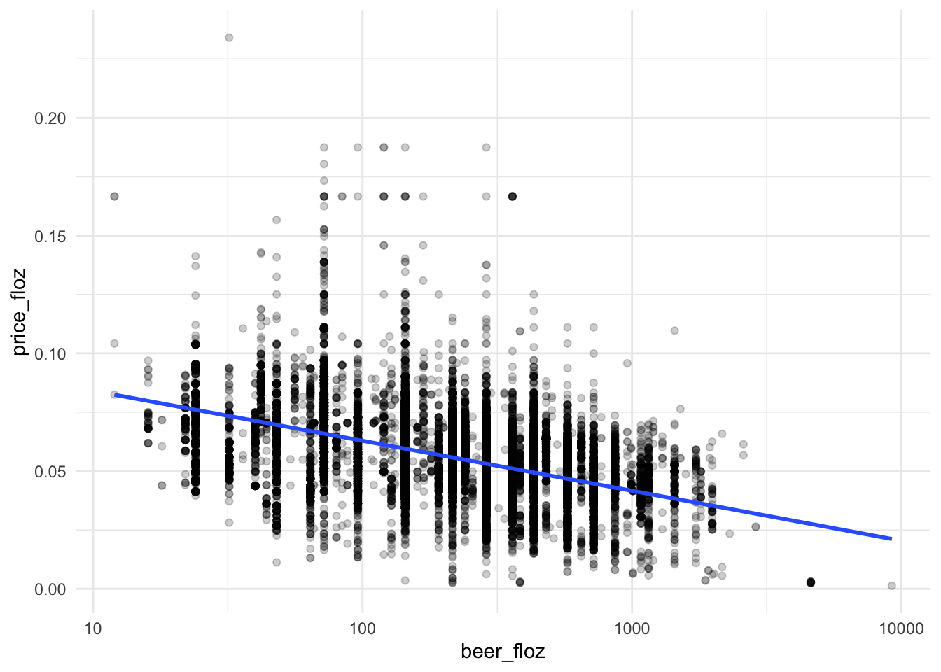
ggplot(beer_markets, aes(x = beer_floz, y = price_floz)) +
  geom_point(alpha = 0.2) +
  geom_smooth(method = "lm") +
  scale_x_log10() +
  theme_minimal()

`geom_smooth()` using formula = 'y ~ x'

After adjusting for extreme bulk purchases using a log scale, the negative relationship between volume and price becomes clearer, suggesting that consumers benefit from lower per-ounce pricing when buying larger quantities.